8.11 Colors
Colors can be set a different way in ggplot2, and in R in general.
8.11.1 All R colors
The easiest way is to fetch colors by their names.
There are 657 color names available for you to pick! You can check them by querying the following in the console:
ggplot2 provides a color scale by default. Many different palettes are available to change the default scale.
8.11.2 Base R palettes
Base R provides built-in palettes, that can be leveraged in ggplot. For example:
- rainbow()
- heat.colors()
- terrain.colors()
- topo.colors()
- cm.colors()
All of the above are functions that take one parameter n i.e. the number of colors needed. The output is a vector of hex color codes, for example:
## [1] "#FF0000" "#CCFF00" "#00FF66" "#0066FF" "#CC00FF"## [1] "#FF0000" "#FF9900" "#CCFF00" "#33FF00" "#00FF66" "#00FFFF" "#0066FF" "#3300FF" "#CC00FF"
## [10] "#FF0099"We can set them as values parameter in the scale_fill_manual() or scale_color_manual() layers:
ggplot(data=gtf, mapping=aes(x=chr, fill=gene_type)) +
  geom_bar(position="dodge") +
  scale_fill_manual(values=rainbow(5))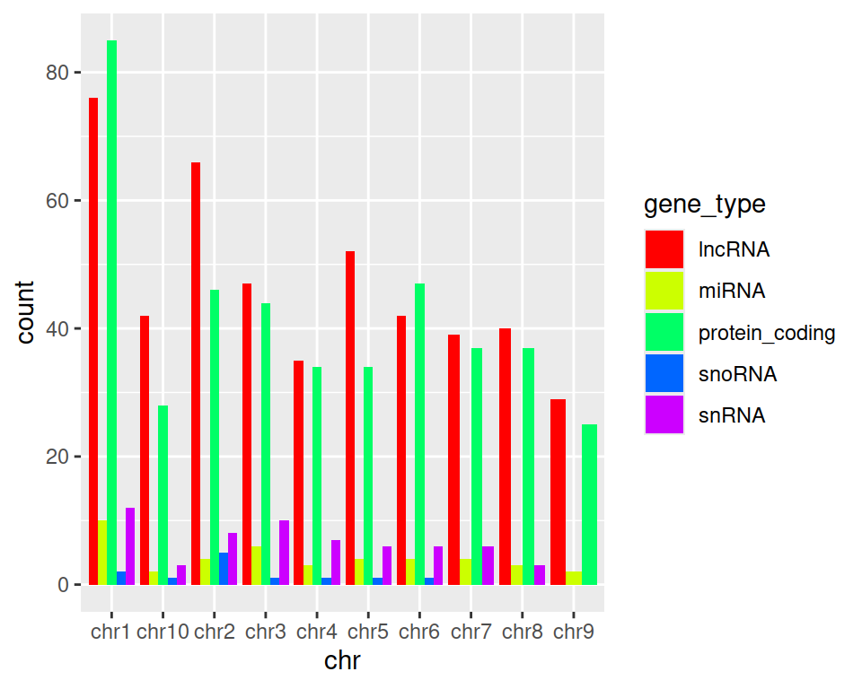
ggplot(data=gtf, mapping=aes(x=chr, fill=gene_type)) +
  geom_bar(position="dodge") +
  scale_fill_manual(values=terrain.colors(5))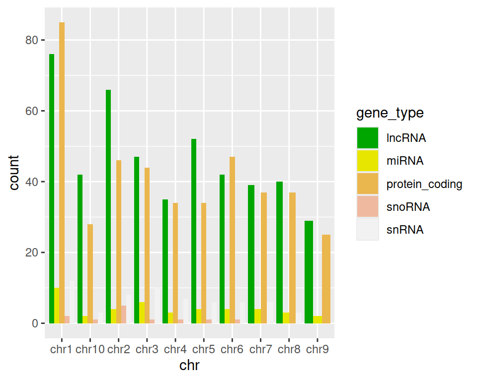
8.11.3 RColorBrewer
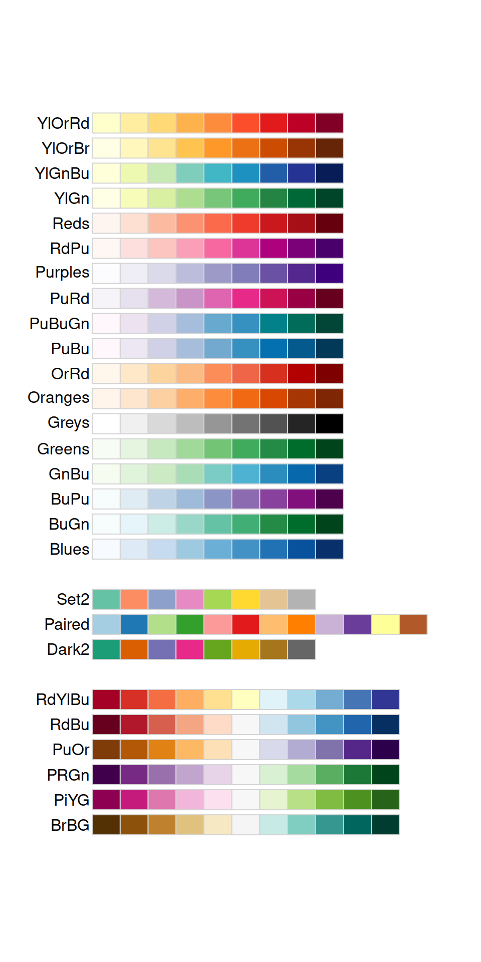
You can easily pick palettes from the RColorBrewer package, that is included in ggplot2.
Available palettes are shown below:
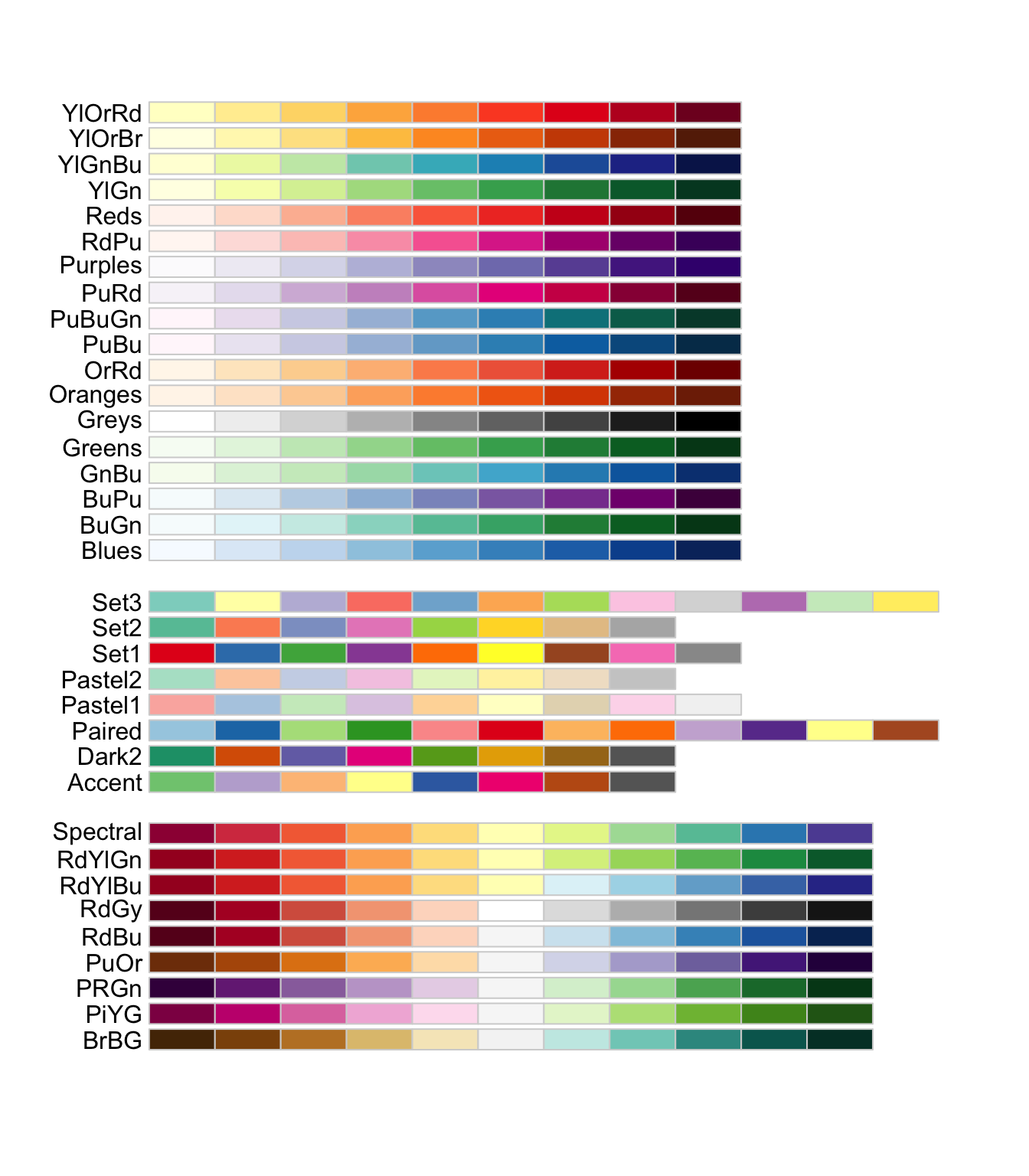
You can check which palettes are colorblind-friendly the following way:
We can easily take advantage of the RColorBrewer’s palettes in ggplot2 with :
- scale_color_brewer() layer (if you mapped variables with color in aes())
- scale_fill_brewer() layer (if you mapped variables with fill in aes())
ggplot(data=gtf, mapping=aes(x=chr, fill=gene_type)) +
  geom_bar(position="dodge") +
  scale_fill_brewer()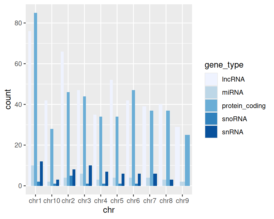
By default, the palette used is “Blues”.
How does that look using “Dark2” palette?
ggplot(data=gtf, mapping=aes(x=chr, fill=gene_type)) +
  geom_bar(position="dodge") +
  scale_fill_brewer(palette="Dark2")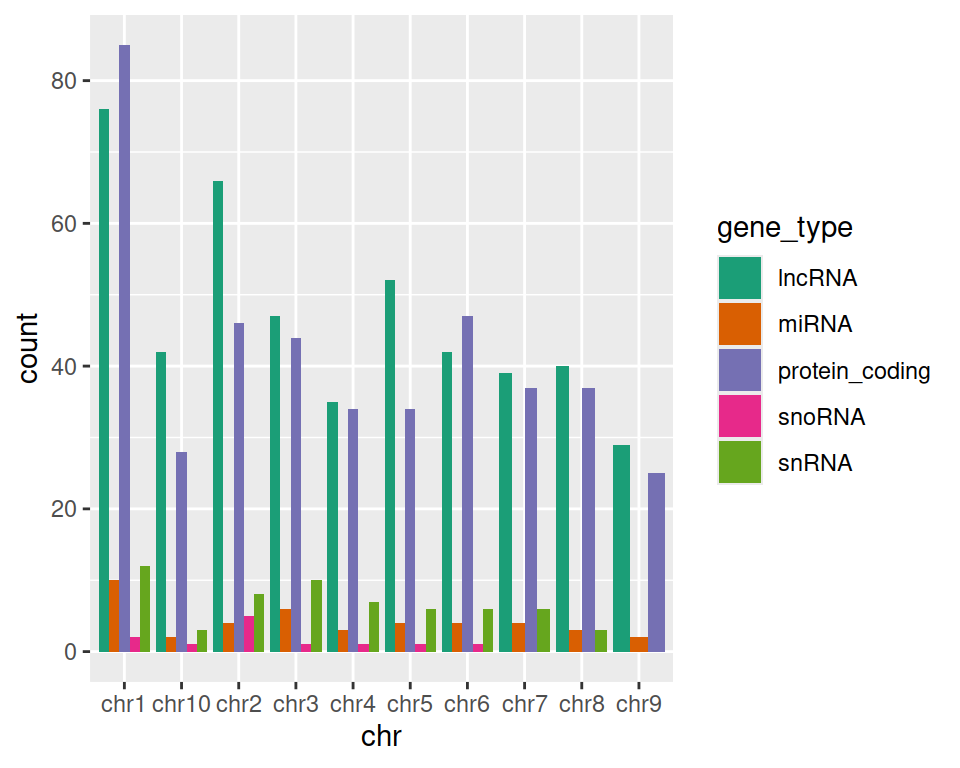
8.11.4 ggsci
Package {ggsci} contains a collection of pre-made color palettes inspired by colors used in scientific journals (and also by Science Fiction movies and series!).
Example of palettes from {ggsci}:
- scale_color_npg() and scale_fill_npg() (Nature Publishing Group)
- scale_color_aaas() and scale_fill_aaas(): (American Association for the Advancement of Science)
- scale_color_lancet() and scale_fill_lancet() (Lancet)
- scale_color_igv() and scale_fill_igv() (Integrative Genome Viewer)
- scale_color_gsea() and scale_fill_gsea() (Gene Set Enrichment Analysis)
- scale_color_startrek() and scale_fill_startrek()
- scale_color_simpsons() and scale_fill_simpsons()
Note that some palettes are for continuous variables (e.g. gsea), and some for discrete variables (e.g. npg).
Example of scales for discrete data:
library(ggsci)

ggplot(data=gtf, mapping=aes(x=chr, fill=gene_type)) +
  geom_bar(position="dodge") +
  ggtitle("scale_fill_ngp", subtitle = "Nature Publishing Group") +
  scale_fill_npg()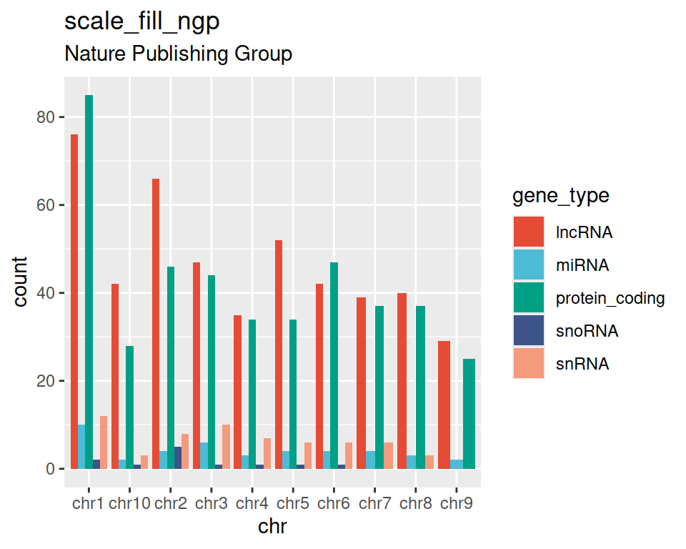
ggplot(data=gtf, mapping=aes(x=chr, fill=gene_type)) +
  geom_bar(position="dodge") +
  ggtitle("scale_fill_aaas", subtitle = "American Association for the Advancement of Science") +
  scale_fill_aaas()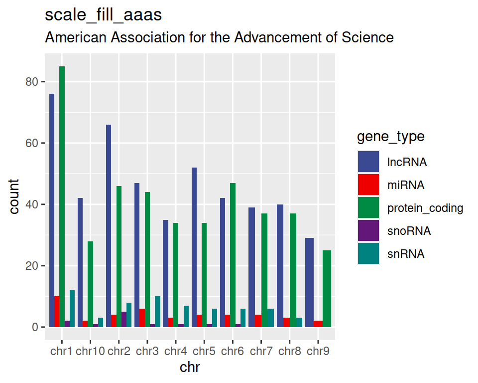
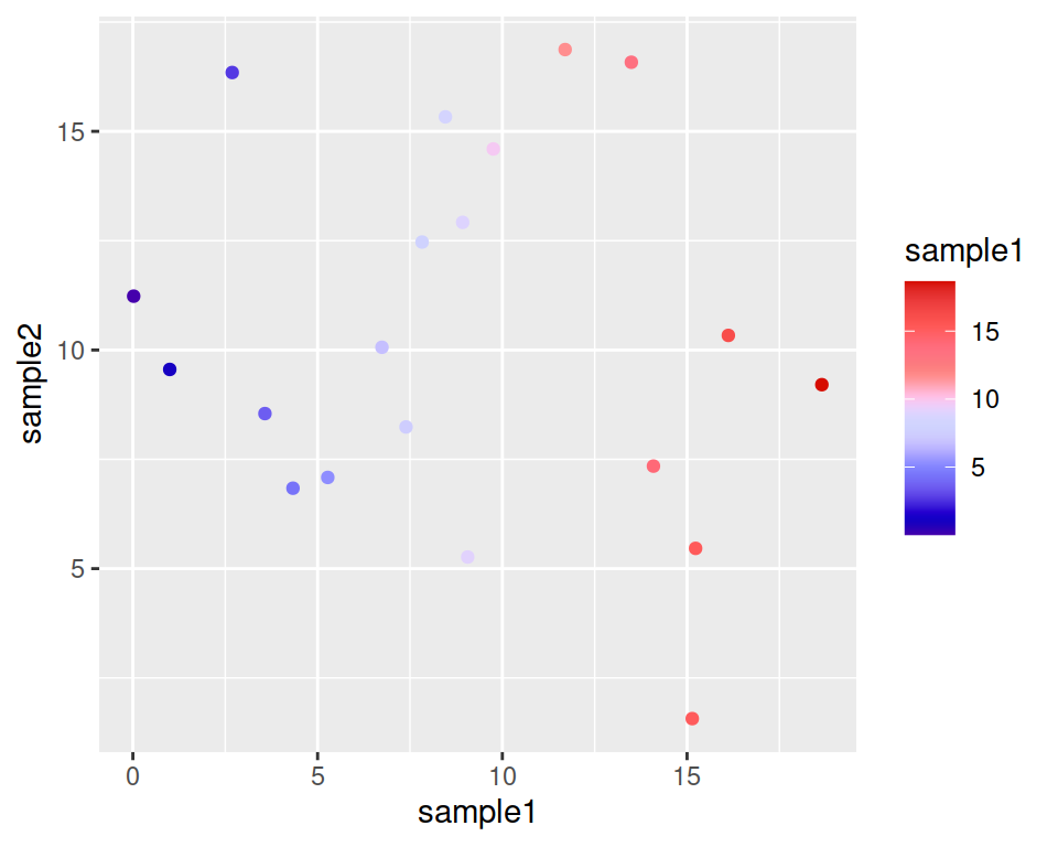
Example of a scale for continuous data:
 ggplot(data=geneexp, mapping=aes(x=sample1, y=sample2, color=sample1)) +
  geom_point() + scale_color_gsea()