8.8 Exercise 2B - review scatter plots before the second day
For this exercise, we will use a built-in dataset iris: this dataset shows data from several flower species.
- Explore dataset: check dim(iris); head(iris); tail(iris)
correction
## [1] 150 5## Sepal.Length Sepal.Width Petal.Length Petal.Width Species
## 1 5.1 3.5 1.4 0.2 setosa
## 2 4.9 3.0 1.4 0.2 setosa
## 3 4.7 3.2 1.3 0.2 setosa
## 4 4.6 3.1 1.5 0.2 setosa
## 5 5.0 3.6 1.4 0.2 setosa
## 6 5.4 3.9 1.7 0.4 setosa## Sepal.Length Sepal.Width Petal.Length Petal.Width Species
## 145 6.7 3.3 5.7 2.5 virginica
## 146 6.7 3.0 5.2 2.3 virginica
## 147 6.3 2.5 5.0 1.9 virginica
## 148 6.5 3.0 5.2 2.0 virginica
## 149 6.2 3.4 5.4 2.3 virginica
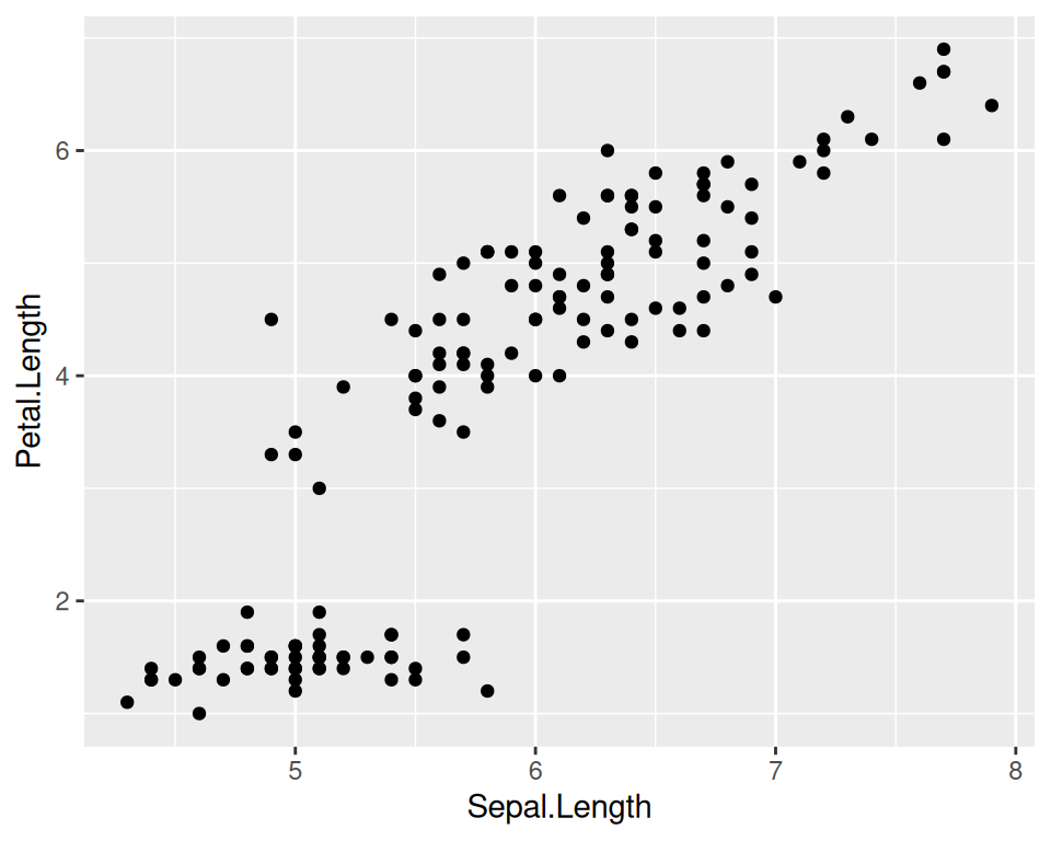
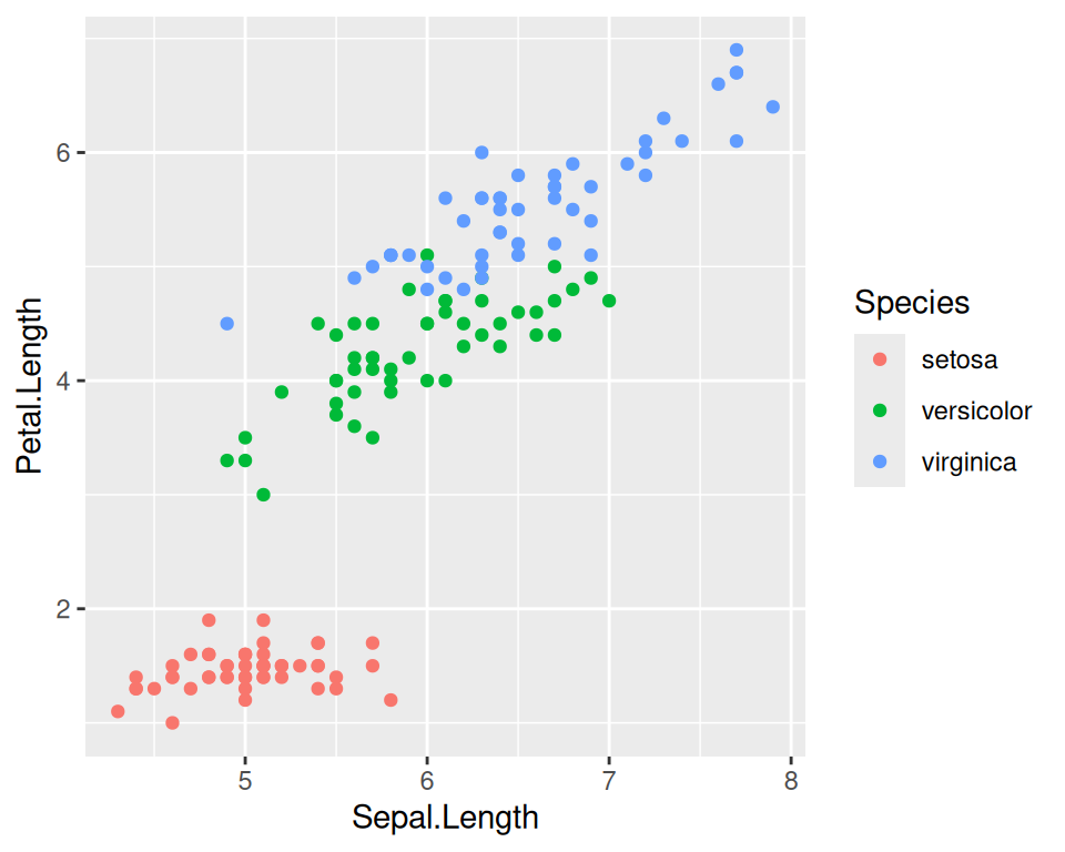
## 150 5.9 3.0 5.1 1.8 virginica- Create a scatter plot of sepal length (x-axis) versus petal length (y-axis)
- Conditionally color points per species
correction
- Add a regression line (or regression lines) to the plot
correction
ggplot(data=iris, mapping=aes(x=Sepal.Length, y=Petal.Length, color=Species)) +
geom_point() +
geom_smooth()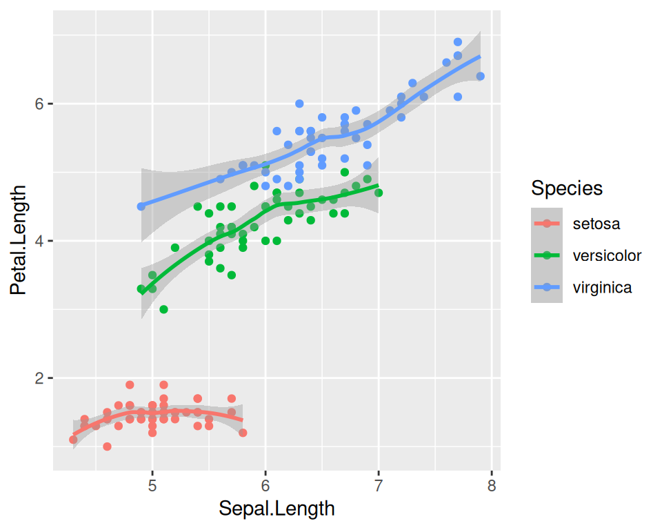
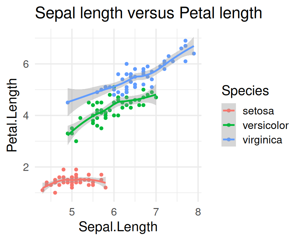
- Change the plot’s default background, add a title, and save plot to a file (either using RStudio interface, or with ggsave() function)
correction
psepal <- ggplot(data=iris, mapping=aes(x=Sepal.Length, y=Petal.Length, color=Species)) +
  geom_point() +
  geom_smooth() +
  theme_minimal(base_size = 16) +
  ggtitle("Sepal length versus Petal length")

plot(psepal)