8.7 Exercise 2
- Import DataViz_source_files-main/files/gencode.v44.annotation.csv in an object that you will call gtf. You can check the first 20 rows of gtf using the head() function: check the help page to see how it works.
correction
The data in gtf represents a small subset of the gencode v44 human gene annotation, created the following way:
- Selection of protein coding genes, long non-coding genes, miRNAs, snRNAs and snoRNAs.
- Selection of chromosomes 1 to 10 only.
- Creation of a random subset of 1000 genes.
- Conversion to a friendly csv format.
## # A tibble: 20 × 5
##    chr   strand gencode_id         gene_type      gene_symbol
##    <chr> <chr>  <chr>              <chr>          <chr>
##  1 chr4  +      ENSG00000250938.8  lncRNA         MAD2L1-DT
##  2 chr4  +      ENSG00000286320.2  lncRNA         ENSG00000286320
##  3 chr1  +      ENSG00000215717.7  protein_coding TMEM167B
##  4 chr3  -      ENSG00000265028.1  miRNA          ENSG00000265028
##  5 chr9  -      ENSG00000242375.1  lncRNA         ENSG00000242375
##  6 chr1  -      ENSG00000143199.18 protein_coding ADCY10
##  7 chr5  +      ENSG00000181751.10 protein_coding MACIR
##  8 chr3  -      ENSG00000290763.1  lncRNA         SDHAP1
##  9 chr8  +      ENSG00000157168.22 protein_coding NRG1
## 10 chr9  +      ENSG00000130956.14 protein_coding HABP4
## 11 chr5  -      ENSG00000250360.1  lncRNA         ENSG00000250360
## 12 chr4  -      ENSG00000250532.1  lncRNA         ENSG00000250532
## 13 chr1  +      ENSG00000067704.10 protein_coding IARS2
## 14 chr10 -      ENSG00000226083.5  lncRNA         SLC39A12-AS1
## 15 chr8  -      ENSG00000136960.13 protein_coding ENPP2
## 16 chr8  +      ENSG00000253263.1  lncRNA         ENSG00000253263
## 17 chr10 +      ENSG00000272381.2  lncRNA         LINC02664
## 18 chr2  +      ENSG00000236854.2  lncRNA         ENSG00000236854
## 19 chr10 -      ENSG00000188716.6  protein_coding DUSP29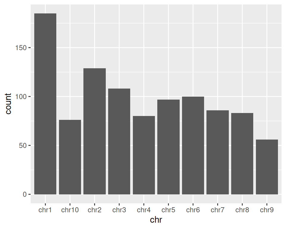
## 20 chr7 - ENSG00000284707.2 lncRNA ENSG00000284707- Create a simple barplot displaying the number of genes per chromosome:
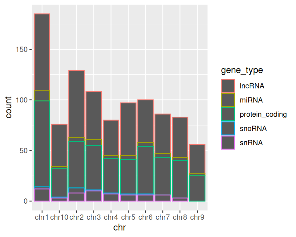
3. Keep chromosomes on the x axis, and split the barplot per gene type.
TIP: remember how we set color= in mapping=aes() function in the scatter plot section? Give it a try here!
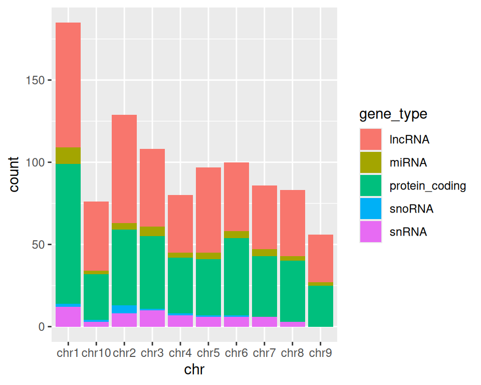
4. Change color= with fill= in aes(). What changes?
5. Add a title to the graph:
correction
ggplot(data=gtf, mapping=aes(x=chr, fill=gene_type)) +
geom_bar() +
ggtitle(label = "Number of genes per chromosome, split by gene type")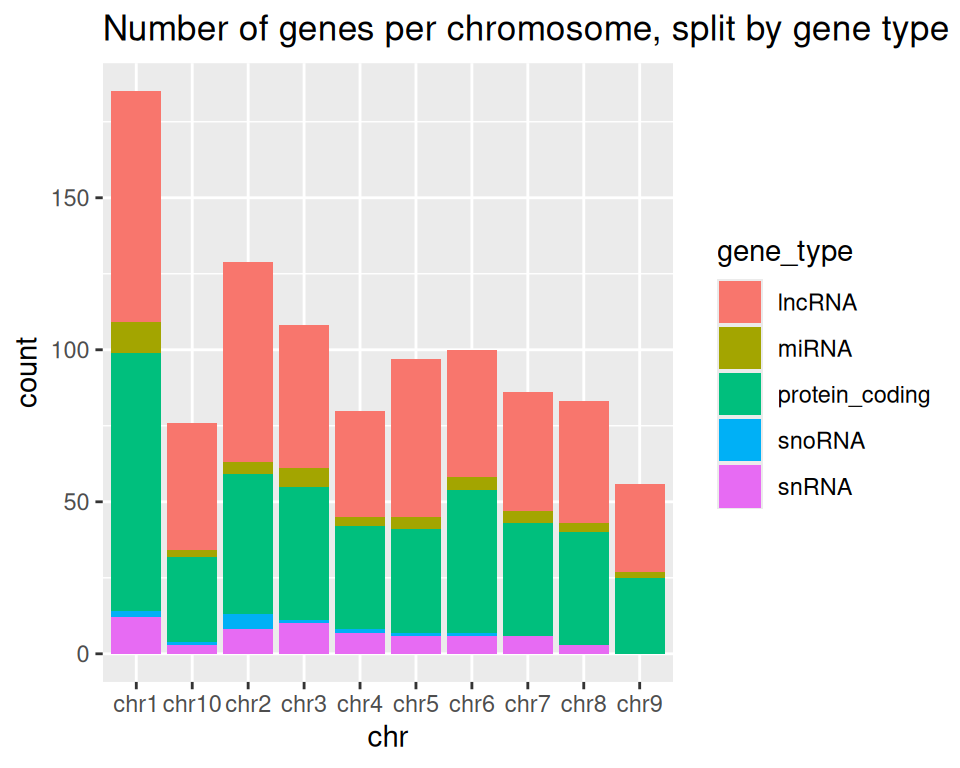
6. Change the default theme:
correction
ggplot(data=gtf, mapping=aes(x=chr, fill=gene_type)) +
  geom_bar() +
ggtitle(label = "Number of genes per chromosome, split by gene type") +
theme_bw()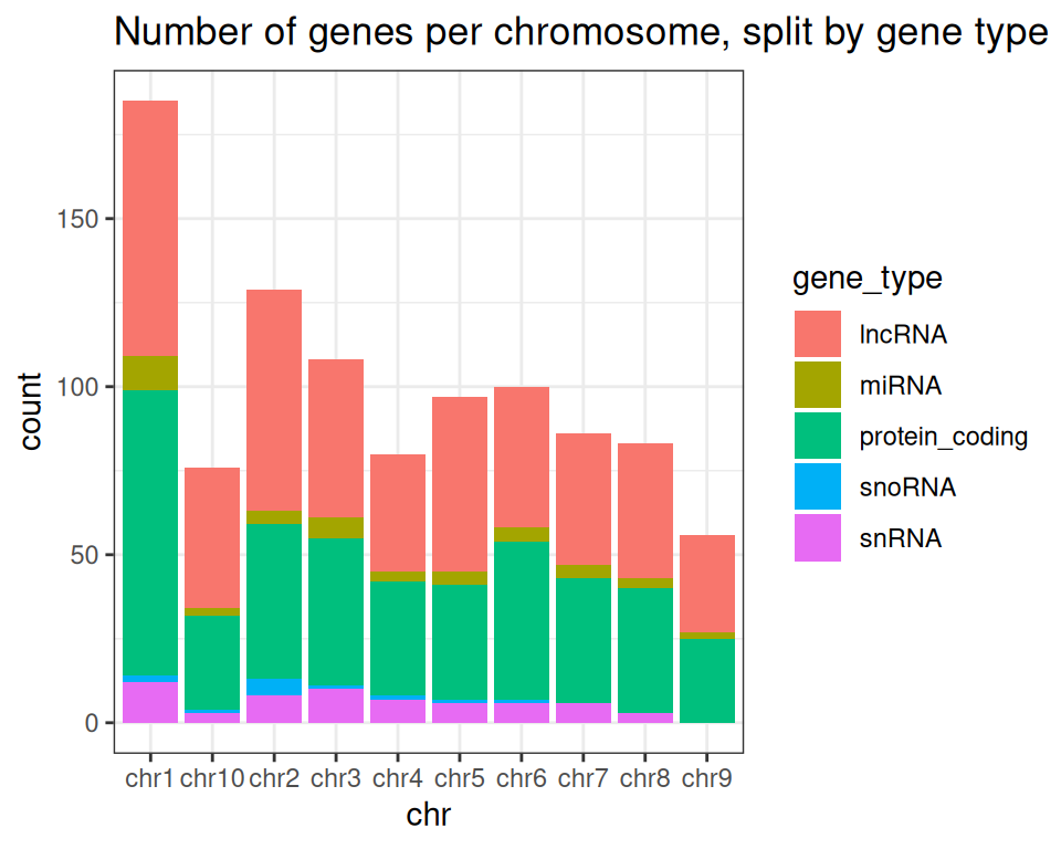
7. Save the graph in PNG format in the workshop’s directory.