8.7 Exercise 2
- Import file DataViz_source_files-main/files/gencode.v44.annotation.csv in R, into an object called gtf.
correction
This is a small subset of the gencode v44 human gene annotation:
- Only protein coding, long non-coding, miRNAs, snRNAs and snoRNAs
- Limited to chromosomes 1 to 10
- Random subset of 1000 genes
- Converted to a friendly csv format.
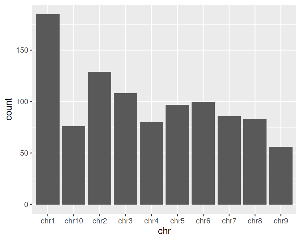
2. Create a simple barplot representing the count of genes per chromosome:
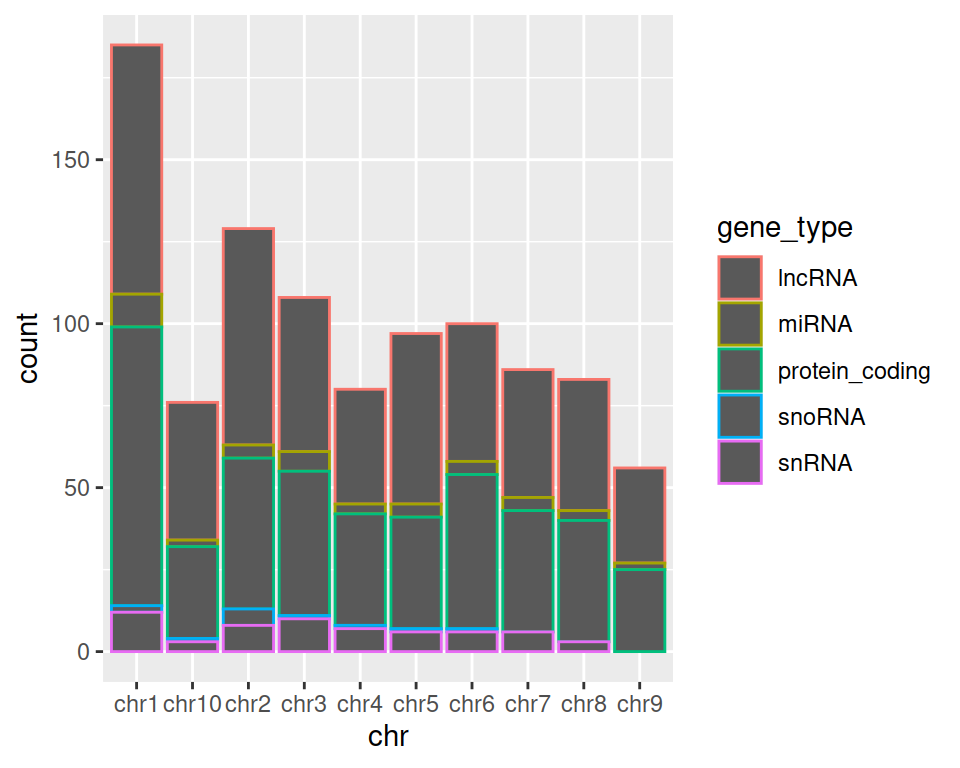
3. Keeping the chromosome on the x axis, split the barplot per gene type.
TIP: remember how we set color= in mapping=aes() function in the scatter plot section? Give it a try here!
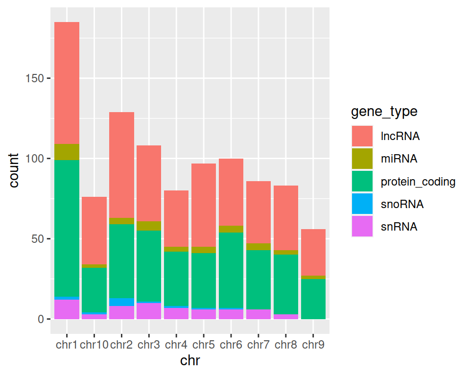
4. Now try with fill instead of color in aes():
5. Add a title to the graph:
correction
ggplot(data=gtf, mapping=aes(x=chr, fill=gene_type)) +
geom_bar() +
ggtitle(label = "Number of genes per chromosome, split by gene type")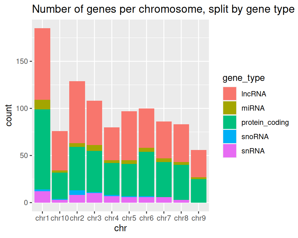
6. Change the default theme:
correction
ggplot(data=gtf, mapping=aes(x=chr, fill=gene_type)) +
  geom_bar() +
ggtitle(label = "Number of genes per chromosome, split by gene type") +
theme_bw()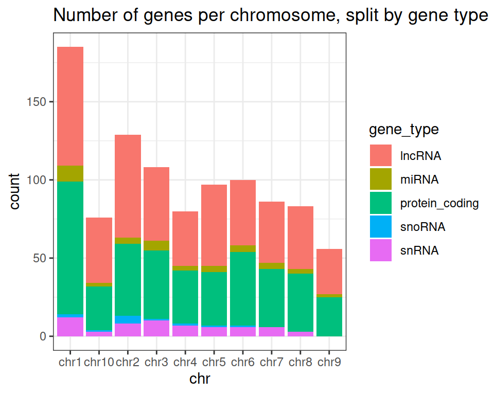
7. Save the graph in PNG format in the course’s directory.